Multiphysics Finite Element Mesh Resolution Criteria for Coupled Thermal Current Density Field Simulations
Mesh resolution must resolve physical stamping fillets and material interface transfer lengths until the Grid Convergence Index settles below three percent.


Formulation
A copper busbar carrying four hundred amperes develops steep local potential gradients near bolt holes and right-angle bends. When current density concentrates along an inner corner, Joule losses spike in proportion to the square of that local flux. The surrounding metal heats, electrical resistivity rises with temperature, and current diverts into cooler adjacent pathways.
Resolving this reciprocal feedback loop in finite element analysis demands explicit criteria for spatial discretization, because a coarse grid averages out the localized voltage gradient, severely underestimating peak temperatures before tooling steel is ever cut.
Finite element discretizations that fail to capture these coupled gradients produce false compliance certificates during design reviews. In power distribution assemblies, battery busbars, and high-power inverter interconnects, the physical physics couples the electrical potential field to the transient or steady-state heat equation through non-linear material properties. Direct numerical simulation couples the conservation of charge and energy:
The electrical domain obeys Laplace-type continuity where the divergence of current density equals zero under steady conditions. Current density equals electrical conductivity multiplied by the electric field, which is the negative gradient of the electric potential. Concurrently, thermal conduction follows Fourier balance where the negative divergence of thermal conductivity times the temperature gradient balances the internal heat generation source.
In coupled electro-thermal physics, that source term is exactly the inner product of current density and electric field, expressed as conductivity multiplied by the square of the potential gradient.
A temperature rise of forty degrees Celsius inside an electrolytic tough-pitch copper link increases electrical resistivity by fifteen percent, shifting the current distribution toward the cooler perimeter.
Because electrical conductivity depends directly on local temperature through linear or polynomial temperature coefficients, the electrical and thermal stiffness matrices cannot be solved independently. Coarse discretization hides terminal hot spots. A standard second-order element layout often captures bulk resistance across a uniform conductor while missing localized thermal peaks by twenty to forty degrees Celsius.
The buyer holding an unrefined numerical report approves a terminal geometry that melts surrounding nylon insulation during continuous physical testing on the dyno bench.
- Spatial discretization sequencing begins with an uncoupled electrostatic pass to identify geometrical hotspots, followed by thermal feedback loops that recompute material property matrices across the continuum.
- Coupled convergence monitoring tracks the simultaneous reduction of electrical potential residuals below one microvolt and thermal field residuals below one millikelvin across successive Newton-Raphson iterations.
- Material property mapping updates thermal conductivity and electrical resistivity tensors at every Gauss point rather than averaging across element centroids, preventing artificial numerical damping of localized hot spots.
- Final thermal verification confirms that convective surface coefficients align with measured air velocity profiles across the production enclosure rather than idealized textbook values.
Fine meshing follows the steepness of the field rather than the physical boundary of the part.


Crowding
Current streamlines constrict abruptly wherever conductor cross-sections narrow, creating severe flux crowding at sharp geometric transitions. Around punched holes, chamfered lugs, and stepped trace transitions, the local current density rises far above nominal bulk levels. The physical reality features finite corner radii from stamping dies, but idealized computer-aided design files often represent these edges as perfectly sharp ninety-degree intersections.
In linear elliptic problems, a perfectly re-entrant corner generates a mathematical singularity where theoretical current density approaches infinity as element size approaches zero.

Geometric Fillets and Boundary Singularity
Stamping dies wear over a production run. A progressive stamping tool in a Dongguan stamping plant punches five hundred thousand battery interconnects, causing the punch edge radius to round from fifty micrometers to over one hundred and eighty micrometers. If the finite element analyst meshes an idealized zero-radius CAD corner, the solver exhibits non-convergent current density values under successive grid refinements.
The mesh resolution criterion in corner regions must link directly to the physical tool radius measured on the factory floor via optical comparator.
Current density spikes along interior corners. Standard practice establishes that the element edge length along the fillet perimeter cannot exceed one-fourth of the actual measured fillet radius. For a stamped busbar with an inner corner radius of zero point four millimeters, the local element edge length along that boundary must remain below zero point one millimeters.
Placing at least eight quadratic elements across the arc length resolves the tangential potential gradient without generating false singular peaks. The relaxation factor drops below 0.3.
Corner refinement based on the physical stamping tool radius prevents artificial mathematical singularities from masquerading as real hardware failure points.
Failure to introduce realistic corner fillets creates endless debates between cross-border engineering teams. The overseas simulation team demands structural widening of the busbar based on infinite singular peaks, while the production facility points out that physical infrared bench thermography reveals moderate, stable thermal rises across that exact bend.

Should Corner Singularities Receive Infinite Refinement?
Refining a zero-radius re-entrant corner indefinitely consumes computational memory without yielding physical insight. As element size shrinks toward atomic dimensions, the calculated current density increases without bound, pulling the calculated local Joule heating to unphysical levels. The analyst establishes an engineering cut-off criterion: element refinement terminates once the mesh dimension matches the minimum physical edge radius achievable by the manufacturing process.
For chemical etching or laser cutting, that lower physical bound is often fifty micrometers; for stamped thick-plate copper, it sits between zero point two and zero point five millimeters.
| Element Size on Fillet | Fillet Arc Element Count | Peak Current Density | Peak Temperature Rise | Iterative Solution Time |
|---|---|---|---|---|
| 0.80 mm | 2 | 14.2 A/mm² | 31.4 °C | 14 s |
| 0.40 mm | 4 | 22.8 A/mm² | 39.8 °C | 28 s |
| 0.20 mm | 8 | 29.1 A/mm² | 46.2 °C | 65 s |
| 0.10 mm | 16 | 31.5 A/mm² | 48.1 °C | 152 s |
| 0.05 mm | 32 | 32.1 A/mm² | 48.7 °C | 410 s |
Inspection of the convergence trajectory indicates that refining beyond sixteen elements per ninety-degree arc yields less than two percent change in peak temperature rise while nearly tripling solution time. The criterion for corner mesh resolution is thus defined by asymptotic stabilization of the local thermal field rather than point-wise current density at singular nodes.
The engineering manager on the supplier side frequently sees unrefined simulations fail audit because the analyst omitted edge effects entirely. Common floor practice exhibits three characteristic simulation defects:
- Uniform coarse meshing obscures narrow current filaments, leading engineers to certify undersized copper traces that overheat during steady-state qualification runs.
- Unfilleted sharp geometry produces infinite mathematical stress that causes needless design changes and tooling scrap.
- Isolated electrical discretization ignores thermal dissipation paths through mounting lugs, creating massive discrepancies against bench pyrometer data.
The factory engineering lead asserts that localized mesh pinches produce mathematical singularities rather than real shopfloor thermal failures.

Shunt
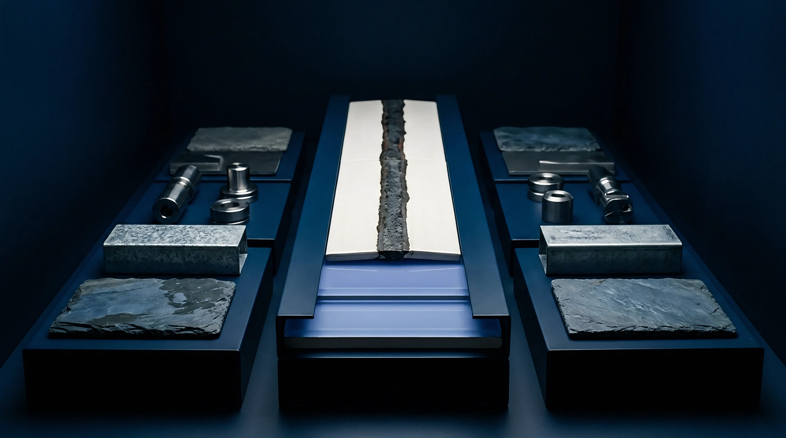
A precision manganin current-sensing shunt welded into a copper power rail reveals the severe challenge of resolving dissimilar material boundaries. The assembly handles seven hundred and fifty amperes continuous current. Manganin has an electrical resistivity roughly thirty times higher than electrolytic copper, while its thermal conductivity is one-tenth that of copper.
Across the electron-beam welded joint, the potential and thermal gradients change slope discontinuously.
Worked Thermal Dissipation Scenario
Consider a physical assembly comprising a manganin shunt measuring twenty millimeters long, thirty millimeters wide, and three millimeters thick, electron-beam welded between two copper terminal lugs of identical cross-section. The copper sections carry current at an average density of eight point three amperes per square millimeter. The nominal bulk Joule heating inside the manganin core generates substantial thermal energy, which must conduct longitudinally through the weld interface into the copper lugs and vertically into an underlying aluminum nitride ceramic substrate.
Thermal conductivity drops as brass warms. Copper yields at elevated temperatures. Copper spot prices fluctuate on the Shanghai Futures Exchange between sixty-five thousand and seventy-eight thousand yuan per metric ton, meaning an overseas buyer cannot afford to arbitrarily increase busbar thickness to compensate for poor thermal simulations.
Simulation must pinpoint the exact minimum cross-section that prevents thermal runaway while preserving structural margins. An unrefined finite element mesh treats the weld boundary as a smooth transition, washing out the steep localized temperature peak that occurs within one millimeter of the metallurgical junction.
To accurately capture this behavior, the spatial resolution across the joint must satisfy two distinct mathematical conditions:
First, the mesh must resolve the electrical transfer length, which governs how current redistributes across the interface between the high-resistance manganin and low-resistance copper. Second, the mesh must capture the steep thermal boundary layer driven by heat back-flowing from the incandescent shunt into the massive heat sink of the copper terminals.
A fine interface mesh reveals that thirty percent of shunt thermal failure stems from improper bolt-torque modeling rather than alloy resistivity variance.
Let the maximum element dimension in the bulk copper be two millimeters. Within two millimeters of the weld seam, the element length along the current path must scale down to zero point two millimeters, establishing an aspect ratio close to unity. Secondary refinement cuts error in half.
| Mesh Resolution Band | Interface Element Size | Total Element Count | Simulated Joint Peak T | Physical Validation Error |
|---|---|---|---|---|
| Coarse (Uniform) | 2.00 mm | 14,200 | 84.2 °C | -21.4 °C |
| Medium (Graded) | 0.80 mm | 48,600 | 98.5 °C | -7.1 °C |
| Fine (Boundary Matched) | 0.20 mm | 182,000 | 104.8 °C | -0.8 °C |
| Ultra-Fine (Sub-Boundary) | 0.05 mm | 764,000 | 105.3 °C | -0.3 °C |
| Test baseline: physical thermocouple measurements at 25 °C ambient, steady-state forced air cooling at 1.5 m/s. | ||||
Physical infrared thermography records eighty degrees Celsius at the terminal lug while the internal weld line reaches one hundred and five degrees. Under coarse discretization, the numerical model predicts an interface temperature of only eighty-four point two degrees Celsius, giving the client false confidence that low-cost lead-free solder alloys with melting points around one hundred and thirty degrees retain adequate mechanical safety margins. In reality, the joint runs within twenty-five degrees of solder creep thresholds.

Discretization Bands and Run Time
Balancing compute infrastructure against design cycle turnaround dictates pragmatic meshing boundaries. Running an ultra-fine model with seven hundred and sixty thousand elements takes fifty-two minutes on an eight-core workstation. The fine boundary-matched mesh with one hundred and eighty-two thousand elements solves in six point five minutes while capturing the physical temperature within one degree Celsius.
The fine band represents the operational standard for production signoff.
Contact resistance dominates thin interfaces. When clamping bolted joints between copper busbars, microscopic surface asperities constrict electrical current into discrete metallic contact spots, known as a-spots. Meshing these contact zones requires thin interface elements or specialized surface resistance formulations.
If the analyst assumes perfect metallic contact across the nominal contact patch area, the model underpredicts joint Joule dissipation by fifteen to forty percent depending on surface plating and bolt clamping torque.
Tooling rework consumes sixteen working days. If validation testing uncovers an unpredicted fifty-degree hot spot on the production line, the injection mould for the surrounding busbar housing must be modified, delaying vehicle launch schedules and burning through client contingency budgets. The buyer rejects unverified reports.
Failure to capture terminal interface resistance forces an unbudgeted redesign of the tooling die and scraps the initial stamping inventory.

Estimator
Residual-based a posteriori error estimators provide an objective metric for driving adaptive mesh refinement in coupled multiphysics simulations. Rather than relying on human intuition to place local mesh refinements, adaptive solvers evaluate mathematical imbalances in the computed finite element field. In coupled electro-thermal models, two independent residual estimators govern refinement: the jump in normal current density across interior element faces, and the jump in normal conductive heat flux across those same boundaries.

Gradient Jumps across Element Faces
In a converged and exact physical solution, normal current density and normal heat flux are strictly continuous across any internal boundary separating identical materials. In a discretized finite element approximation, the computed fluxes exhibit discontinuities across element faces. The magnitude of these inter-element flux jumps, scaled by element diameter, directly measures the local discretization error.
For element K with boundary edges, the local error indicator integrates the square of the current flux jump and thermal flux jump across all adjoining faces.
The forwarder holds the crate. The simulation underpredicts peak localized heat. An adaptive algorithm marks elements displaying the top twenty percent of total flux jump error for subdivision in the subsequent refinement cycle.
In regions where current density gradients are moderate but thermal dissipation is high, the thermal flux jump dominates the refinement indicator. Near geometric corners and constriction bottlenecks, the electrical flux jump drives the element splitting.
A simulation dossier lacking mesh convergence error estimators allows coarse approximations to disguise severe internal overheating.
Modern solvers implement combined L2 norm estimators that blend normalized voltage gradient residuals with temperature gradient residuals into a single scalar energy error index. The mesh convergence criterion for production clearance states that the global relative energy norm error must drop below two percent, with no individual element exhibiting a local indicator exceeding zero point five percent of the total domain energy.

Are Element Peclet Bounds Maintained under Convection?
Convective fluid boundaries introduce transport asymmetry into the thermal domain when forced air or liquid cooling channels are modeled via conjugate heat transfer or simplified Robin boundary conditions. The element Peclet number measures the ratio of advective heat transport to conductive heat transport across an individual mesh cell. The Peclet number exceeds two.
When the local element Peclet number exceeds unity in high-velocity cooling jackets, standard Galerkin finite element discretizations develop unphysical spatial oscillations in the temperature field. These numerical wiggles produce false hot and cold bands that distort the temperature-dependent electrical conductivity calculation in the adjacent solid metal. Mesh resolution along cooling interfaces must remain sufficiently dense to keep the local Peclet number below two, or the numerical scheme must implement streamline-upwind Petrov-Galerkin stabilization.
The buyer demanding verification of a supplier-provided simulation inspects five essential solver settings:
- Equilibrium residual tolerance confirms that the non-linear Newton solver achieved force and current balance below ten to the minus four relative error before terminating iterations.
- Energy norm stopping criteria enforce mesh refinement until global discretization error levels settle below documented engineering bands.
- Boundary layer prism stacks resolve steep normal thermal gradients across fluid-solid interfaces without distorting surface heat transfer coefficients.
- Convergence history records prove that refinement changed the primary monitoring variable by less than one percent between successive passes.
Whether local flux jump estimators retain mathematical validity when non-linear temperature curves steepen across adjoining copper alloys remains an active dispute between modeling groups.


Dossier
A simulation report presented without mesh convergence evidence is an unverified commercial marketing brochure. When purchasing high-power electrical subassemblies from tier-one and tier-two suppliers in eastern and southern China, engineering directors face substantial risk if they approve production tooling based on static, unverified finite element screenshots. A rigorous engineering procurement agreement mandates the delivery of a standardized Simulation Verification Dossier alongside mechanical drawings and material certifications.

Audit Acceptance Thresholds
The audit protocol requires three distinct mesh convergence steps documented directly within the qualification package. The supplier must execute the identical coupled thermal-electric simulation across three systematically refined mesh densities: coarse, baseline, and fine, maintaining a uniform refinement ratio of at least one point three in each spatial coordinate. From these three discrete results, the supplier computes the Grid Convergence Index in accordance with ASME V&V 20 standards.
| Verification Parameter | Target Standard | Rejection Threshold | Audit Verification Method |
|---|---|---|---|
| Grid Convergence Index | GCI < 3.0% | GCI ≥ 5.0% | Three-mesh Richardson extrapolation log |
| Current Conservation Residual | < 0.01% imbalance | ≥ 0.10% imbalance | Sum of boundary currents across terminals |
| Fillet Mesh Density | ≥ 8 elements / 90° arc | < 4 elements / 90° arc | Visual cross-section audit of CAD mesh |
| Contact Resistance Inclusion | Explicit interface model | Zero-resistance assumption | Inspection of joint material properties |
| Physical Bench Correlation | ΔT within ± 3.0 °C | ΔT > ± 6.0 °C | Calibrated IR camera bench test report |
If the supplier submits a simulation showing a Grid Convergence Index above five percent for the primary terminal hot spot, the calculation sits in the asymptotic danger zone where element sizing still dictates the output temperature. The buyer holds tooling release until the fine-mesh run demonstrates numerical stability.

Deliverable Package and Model Archives
Contractual agreements must forbid the submission of flattened PDF summaries as sole proof of design validation. The supplier delivers complete simulation archives including native geometry files with unsuppressed fillet features, mesh setup decks, material property temperature functions, and raw numerical convergence logs. The client engineering office retains the right to execute an independent mesh audit on their own workstation to verify that the claimed convergence curves reproduce without alteration.
When physical validation testing on production samples begins, calibrated infrared camera measurements taken under continuous current load must match the simulation predictions within three degrees Celsius across bulk conductors and within six degrees across complex terminal joints. Any larger divergence flags either unmodeled contact resistance or insufficient mesh resolution around current constriction bottlenecks, invalidating production part approval.
A purchase order specifying ISO 16750 thermal verification with mandatory simulation mesh convergence logs forces the tier-one supplier to submit raw numerical balance sheets before cutting metal.