Constructing Intersecting Diffusion Paths for Multicomponent Interdiffusion Matrix Inversion
Inverting multicomponent interdiffusion matrices requires two couples crossing at angles above 40 degrees to keep gradient condition numbers below 15.


Inversion
Multicomponent diffusion couples trace compositional trajectories across phase diagrams to extract Onsager phenomenological coefficients. Determining the four composition-dependent coefficients of a ternary system requires two independent diffusion paths that cross at an identical composition coordinate. A single diffusion couple yields only two independent flux equations at any given point along its penetration distance, which leaves the four-coefficient interdiffusion matrix mathematically underdetermined.
Two couples resolve four unknowns.
Operating metallurgical laboratories in Jiangsu and Shaanxi frequently fabricate arbitrary diffusion couples without calculating crossing trajectories beforehand. When two couples fail to intersect within the single-phase field, matrix inversion becomes mathematically impossible at the desired composition. The client team loses four to six weeks of vacuum furnace time and metallographic preparation before microprobe data reveals the non-intersecting paths.

Mathematical Prerequisites for Matrix Determination
Phenomenological flux equations define the rate of transport relative to the volume-fixed frame of reference. For a ternary system comprising components 1, 2, and solvent 3, the interdiffusion fluxes J̃1 and J̃2 depend directly on both concentration gradients:
J̃1 = – D̃113 (∂C1/∂x) – D̃123 (∂C2/∂x)
J̃2 = – D̃213 (∂C1/∂x) – D̃223 (∂C2/∂x)
Evaluating the four interdiffusion coefficients D̃113, D̃123, D̃213, and D̃223 at a specific composition C0 = (C10, C20) demands four independent algebraic equations. Couple A provides two equations relating its measured fluxes to its local concentration gradients. Couple B provides two additional equations relating its measured fluxes to its distinct concentration gradients at that exact composition.
The resulting linear system organizes into two decoupled matrix pairs sharing a common gradient coefficient matrix G:
= –
= –
Inversion requires that the determinant of matrix G remains distinctly nonzero. The determinant equals zero.
Collinear or parallel concentration gradients force the determinant to zero, rendering matrix inversion undefined. Experimental success hinges upon forcing the two concentration profile vectors to intersect at an angle sufficiently wide to stabilize numerical inversion against analytical measurement scatter.

Geometric Alignment across the Gibbs Triangle
Phase equilibria and terminal end-member compositions govern the trajectory of a diffusion path through ternary space. Selecting terminal alloys by intuition leads to parallel paths or intersections located outside the target composition domain.
- Terminal alloy composition span isolates the targeted intersection coordinate within the central third of both diffusion vectors.
- Diffusional path curvature estimation utilizes preliminary mobility data or DICTRA simulations to predict serpentine deviations caused by strong thermodynamic interactions.
- Single-phase solid solution limits prevent the diffusion trajectory from crossing two-phase tie-lines where discontinuous concentration steps destroy gradient continuity.
- Molar volume parity between terminal end members minimizes Kirkendall porosity and prevents plastic deformation from distorting the one-dimensional diffusion geometry.
Constructing intersecting paths begins with arc-melting four high-purity terminal buttons. Each button undergoes vacuum homogenization for 120 hours at 1473 Kelvin to eliminate dendritic microsegregation. Chemical assays via inductively coupled plasma optical emission spectrometry verify that bulk compositions match nominal targets within 0.15 atomic percent.
A composition deviation of 0.5 atomic percent shifts the resulting diffusion trajectory by tens of micrometers in composition space, completely bypassing the planned intersection point.
A missed intersection invalidates the entire experimental batch, writing off the initial lab retainer and delaying down-selection by two complete furnace cycles.

Clamp
Mechanical bonding fixtures maintain uniaxial compressive stress during the initial transient of solid-state contact. Achieving intimate metallic contact between two alloy blocks without inducing macroscopic plastic deformation demands calibrated loading mechanics. Excess mechanical stress causes lateral extrusion of softer terminal phases, destroying the planar reference boundary required for Matano coordinate calculations.
Surface roughness exceeds 50 nanometers.
Oxide films, machining gouges, or non-parallel bonding faces generate microscopic voids across the interface. These voids act as internal sinks for vacancy condensation during high-temperature annealing, splitting the diffusion front into irregular, three-dimensional pathways that violate one-dimensional Fickian transport assumptions.
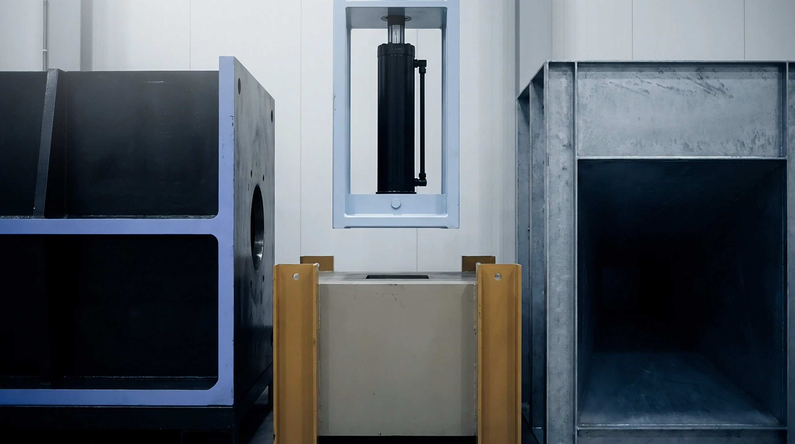
Mating Faces and Boundary Planarity
Precision wire electrical discharge machining sections homogenized alloy ingots into rectangular blocks measuring 10 by 10 by 5 millimeters. The opposing bonding faces must achieve optical planarity before thermal assembly.
- Mechanical silicon carbide grinding advances through 400, 800, and 1200 grit papers under continuous ethanol lubrication to eliminate damaged surface layers.
- Diamond suspension polishing utilizes 3-micrometer and 1-micrometer diamond pastes on low-nap cloths to establish uniform flatness across the metallic contact face.
- Colloidal silica polishing removes sub-surface residual cold work using a 0.04-micrometer alkaline silica suspension for 45 minutes per face.
- Interferometric planarity verification confirms face curvature remains below one interference fringe across the entire contact surface.
The operator discards the couple.
Interfacial cleanliness dictates contact bonding kinetics. Degreasing proceeds through sequential ultrasonic baths of acetone, high-purity ethanol, and deionized water. Polished surfaces exposed to ambient air develop passivating native oxide layers within thirty minutes.
Mating blocks enter the bonding fixture immediately following vacuum desiccation.
A bonding preload exceeding 18 megapascals at 1173 Kelvin causes lateral barreling greater than 1.5 percent plastic strain.

Torque Application during Solid State Assembly
Bonding assemblies utilize high-purity molybdenum or TZM alloy clamping blocks. Differential thermal expansion between the specimen alloys and the clamping frame supplies the sealing pressure during the initial heat ramp.
| Fixture Material | Thermal Expansion Coefficient (10^-6 / K) | Yield Strength At 1273 K (MPa) | Vacuum Creep Rate (1/s at 20 MPa) | Interfacial Carburization Risk |
|---|---|---|---|---|
| High-Density Graphite | 4.2 | 45 | 2.1 x 10^-7 | Severe without barrier foil |
| TZM Molybdenum Alloy | 5.4 | 285 | 4.5 x 10^-8 | Negligible |
| Pure Tungsten Rig | 4.5 | 310 | 1.2 x 10^-8 | None |
| 310S Stainless Steel | 18.5 | 22 | 8.6 x 10^-5 | Moderate cross-diffusion |
Tightening torque on fixture bolts requires calibrated torque wrenches to set initial room-temperature seating pressure. Belleville spring washers made of high-temperature nickel alloys absorb transient thermal spikes, maintaining contact pressure between 10 and 15 megapascals throughout the 30-minute bonding cycle at 1173 Kelvin.
Interfacial strain reaches three percent.
Bonding in a vacuum hot press operating below 5 x 10^-4 Pascals prevents interfacial oxidation. The heating cycle ramps at 10 Kelvin per minute to avoid thermal shock cracking along brittle intermetallic interfaces. Once bonded, the assembly releases from the clamping jig before high-temperature diffusion annealing begins.
Leaving the couple clamped during extended thermal exposure introduces continuous stress fields that bias vacancy flux and distort chemical diffusion coefficients.
The contract machine shop insisted that standard surface grinding without colloidal polishing would weld cleanly under furnace pressure.
Furnace
Isothermal thermal exposures demand tight vacuum levels and negligible thermal gradients to satisfy analytical boundary conditions. Interdiffusion coefficients follow an Arrhenius temperature dependence: D̃ = D0 exp(-Q / RT). An uncorrected furnace temperature deviation of five Kelvin shifts calculated diffusion coefficients by twelve to eighteen percent in nickel-base and cobalt-base superalloy matrices at 1373 Kelvin.
Thermocouple drift exceeds three Kelvin.
Extended annealing schedules range from 48 to 600 hours depending on the refractory content of the target multicomponent system. Furnace hot zones experiencing thermal drift, localized power fluctuations, or uneven element degradation invalidate the isothermal assumption required by Boltzmann-Matano integration.

Thermal Stability across Long Duration Runs
Annealing runs rely on multi-zone horizontal tube furnaces equipped with proportional-integral-derivative controllers. Type S platinum-rhodium thermocouples measure hot-zone temperatures, recalibrated against pure gold melting standards every 300 operating hours. Ceramic processing facilities in Zhejiang often substitute Type K thermocouples for high-temperature runs to cut costs.
Standard Type K couples degrade rapidly above 1273 Kelvin, drifting downward by as much as 15 Kelvin over a 200-hour exposure while reporting nominal stability.
The technician halts the run.
Temperature gradients across the specimen zone must not exceed 0.5 Kelvin over a 50-millimeter span. A three-point thermocouple profiling array placed directly adjacent to the specimen encapsulates the thermal history. Continuous datalogging records hot-zone stability at one-minute intervals throughout the multi-week anneal.
ASTM E228 thermal validation clauses invalidate interdiffusion data sets derived from thermal runs exhibiting temperature variations greater than plus or minus 1.0 Kelvin from the setpoint.
Atmospheric Control and Quartz Encapsulation
High vapor pressure elements like chromium, manganese, and zinc volatilize rapidly at elevated annealing temperatures under direct high vacuum. Evaporative loss changes the terminal alloy composition at the specimen edges, establishing long-range vapor transport that destroys the semi-infinite boundary conditions of the diffusion couple.
| Thermal Envelope (K) | Atmospheric Condition | Activation Energy Q (kJ/mol) | Coefficient Variance (%) | Compositional Shift At Matano Interface (at.%) |
|---|---|---|---|---|
| +/- 0.5 | Argon backfill (25 kPa) | 280 | 1.2 | 0.02 |
| +/- 2.0 | Argon backfill (25 kPa) | 280 | 4.9 | 0.08 |
| +/- 5.0 | Continuous Dynamic Vacuum | 280 | 12.8 | 0.35 |
| +/- 10.0 | Roughing Vacuum (1 Pa) | 280 | 27.4 | 1.10 |
| Calculations assume pure ternary single-phase face-centered cubic matrix with baseline diffusivity D_tilde = 1.0 x 10^-14 m^2/s. | ||||
Specimens reside inside fused quartz capsules evacuated to 2 x 10^-5 Pascals. Chemical cleaning of the quartz tubes involves hydrofluoric acid etching followed by high-temperature baking at 1273 Kelvin for two hours to drive off residual hydroxyl groups. A high-purity titanium or zirconium sponge getter sits inside the sealed capsule, isolated from the diffusion specimen by a quartz wool plug.
Argon backfill pressure reaches 20 kilopascals.
Backfilling the capsule with ultra-high purity argon to 20 kilopascals prevents atmospheric quartz collapse at temperatures above 1373 Kelvin while suppressing volatile element sublimation. Quenching terminates the diffusion anneal. The capsule drops into ice water within two seconds of furnace extraction, shattering the quartz to freeze high-temperature vacancy distributions and arrest non-isothermal interdiffusion during cooling.
Thermal stability over weeks of exposure matters far more than rapid furnace ramp rates.

Microprobe
Wavelength dispersive spectrometers record spatial intensity profiles across polished metallurgical mounts. Converting raw X-ray counts into accurate elemental concentration profiles demands systematic background subtraction, dead-time corrections, and rigorous matrix parameter adjustments. Electron probe microanalysis (EPMA) line scans provide the primary numerical data from which interdiffusion fluxes and spatial gradients emerge.
The beam diameter measures one micrometer.
Broad beam interaction volumes obscure steep concentration gradients near the Matano interface. When spatial step sizes exceed the local diffusion penetration depth, finite difference gradient approximations introduce massive numerical errors into the inversion matrix.

Spatial Step Selection and Interaction Volume
Operating parameters dictate analytical spatial resolution. An accelerating voltage of 15 kilovolts with a probe current of 30 nanoamperes provides an optimal balance between X-ray yield and interaction volume containment. Monte Carlo electron trajectory simulations show that beam excitation in a nickel-cobalt-chromium matrix spreads across a lateral diameter of 0.85 micrometers under these conditions.
- Spatial step spacing maintains a minimum interval of 1.0 micrometer to prevent overlapping beam damage while capturing at least 80 discrete data points across the interdiffusion zone.
- Pure element calibration standards undergo beam current normalization before and after each linear trace to compensate for filament emission drift.
- Diffraction crystal selection pairs high-resolution lithium fluoride crystals with transition metal K-alpha lines to resolve peak overlaps between adjacent atomic numbers.
- Counting time per point exceeds 30 seconds on peak and 15 seconds on background to suppress Poisson counting noise below 0.2 percent relative uncertainty.
Automated stage movements drive the specimen perpendicular to the bonded interface. Tilting or skewing the scan line relative to the diffusion normal artificially stretches the measured diffusion distance, introducing geometric cosine errors into the spatial coordinate x.
Smooth spline fits must match raw concentration data without introducing artificial oscillations into the first spatial derivatives.
Gradient Extraction and Matano Plane Integration
Extracting interdiffusion fluxes requires establishing the Matano coordinate x0 for each individual couple. The Matano plane location satisfies mass balance conservation across the diffusion zone:
∫-∞x0 (Ci – Ci–) dx = ∫x0+∞ (Ci+ – Ci) dx
Here Ci– and Ci+ denote the terminal boundary compositions at negative and positive infinity. Raw concentration data exhibit analytical scatter that destabilizes direct numerical differentiation. Fitting raw data with tension splines or piecewise analytic error-function expansions smooths the profiles prior to differentiation.
Take a worked ternary nickel-cobalt-chromium construction at 1373 Kelvin. Couple A bridges Ni-10Co-20Cr against Ni-40Co-5Cr, while Couple B bridges Ni-30Co-25Cr against Ni-20Co-0Cr. The diffusion paths intersect at Ni-25Co-12.5Cr (atomic percent).
Numerical integration of Couple A yields fluxes J̃CoA = -1.45 x 10^-11 mol/(m^2 s) and J̃CrA = 8.20 x 10^-12 mol/(m^2 s), with local concentration gradients (dCCo/dx)A = 1.85 x 10^5 mol/m^4 and (dCCr/dx)A = -1.10 x 10^5 mol/m^4.
Couple B yields fluxes J̃CoB = -6.10 x 10^-12 mol/(m^2 s) and J̃CrB = 1.55 x 10^-11 mol/(m^2 s), with measured gradients (dCCo/dx)B = 0.65 x 10^5 mol/m^4 and (dCCr/dx)B = 1.95 x 10^5 mol/m^4.
Constructing the gradient matrix G yields:
G =
The determinant evaluates directly: Det(G) = (1.85 x 10^5)(1.95 x 10^5) – (-1.10 x 10^5)(0.65 x 10^5) = 3.6075 x 10^10 + 0.715 x 10^10 = 4.3225 x 10^10 mol^2/m^8. Inverting the system extracts the full interdiffusion matrix at the intersection coordinate: D̃CoCoNi = 7.24 x 10^-16 m^2/s, D̃CoCrNi = -1.02 x 10^-16 m^2/s, D̃CrCoNi = -2.15 x 10^-16 m^2/s, and D̃CrCrNi = 7.18 x 10^-16 m^2/s.
Whether secondary fluorescent excitation across sharp concentration steps distorts derivative values near the Matano interface remains an active debate among microprobe analysts.

Conditioning
Matrix inversion sensitivity depends directly on the angle subtended by the crossing concentration vectors. When two diffusion paths cross at an acute angle in the Gibbs triangle, the rows of gradient matrix G approach linear dependency. Numerical inversion under these conditions magnifies microprobe counting noise into massive oscillations across off-diagonal diffusion coefficients.
The crossing angle measures twelve degrees.
A poorly conditioned gradient matrix frequently produces unphysical results, such as negative main interdiffusion coefficients or cross-coefficients that violate Onsager thermodynamic stability criteria: D̃11 D̃22 – D̃12 D̃21 > 0. Laboratory quality control programs must calculate the condition number of G before accepting inverted kinetic parameters.
Crossing Geometry and Determinant Collapse
The crossing angle θ between diffusion paths A and B in composition space reflects the scalar product of their normalized gradient vectors:
cos(θ) = /
As the crossing angle drops below 20 degrees, the determinant of G plummets toward zero, causing the condition number cond(G) = ||G|| ||G^-1|| to escalate exponentially.
| Crossing Angle (degrees) | Gradient Matrix Determinant (arbitrary units) | Condition Number cond(G) | Propagated Main Coefficient Error (%) | Propagated Cross Coefficient Error (%) |
|---|---|---|---|---|
| 85 | 0.996 | 1.2 | 1.5 | 3.2 |
| 60 | 0.866 | 2.4 | 2.8 | 6.5 |
| 35 | 0.573 | 5.8 | 6.4 | 18.5 |
| 15 | 0.258 | 24.5 | 28.0 | 85.0 |
| 5 | 0.087 | 145.0 | 160.0 | 520.0 |
The condition number reaches 180.
A condition number exceeding 20 indicates severe ill-conditioning. A minor microprobe measurement uncertainty of 1.0 percent propagates through an ill-conditioned system to yield an 85 percent error margin in the cross-coefficients D̃12 and D̃21. Cross-coefficients dictate diffusional interaction and uphill diffusion behavior, making precise extraction vital for kinetic modeling in multi-component alloy development.
The laboratory reruns both couples.
Crossing angles greater than 40 degrees suppress numerical noise amplification during interdiffusion matrix inversion.

Laboratory Acceptance Thresholds and Commercial Retainers
Commercial metallurgical laboratories frequently deliver raw microprobe traces without performing matrix inversion verification. By delegating the numerical inversion to the client, the facility obscures failed crossings and defective thermal runs behind standard raw-data delivery certificates. Once the final invoice closes, recovering costs for uncrossed or ill-conditioned diffusion couples becomes nearly impossible.
The buyer withholds final payment.
Managing cross-border metallurgical testing requires restructuring laboratory service level agreements. Payment terms must divide fees into three distinct milestone deliverables: 30 percent upon metallographic validation of void-free bonded interfaces, 30 percent upon verified isothermal furnace datalogs and quenched specimen delivery, and 40 percent upon successful extraction of the interdiffusion matrix with a verified gradient condition number below 15.
Milestone payment schedules tied directly to matrix condition metrics shift financial accountability back to the testing facility, eliminating unverified microprobe deliverables from international R&D budgets.